Do you wanna know What is Gradient Descent in Neural Network ?, Its role in Neural Network?. Give your few minutes to this blog, to understand the Gradient Descent Neural Network completely in a super-easy way. You will understand the Gradient Descent Neural Network in a few minutes. So read this full article :-).
Hello, & Welcome!
In this blog, I am gonna tell you-
- How does Neural Network Learn?
- What is Gradient Descent?
Gradient Descent Neural Network
In order to understand Gradient Descent, first, you need to know how a neural network learns?. So first I will explain to you the whole process of neural network learning.
So without wasting your time, let’s get started-
How does Neural Network Learn?
As I have discussed in my previous articles that in Neural Network you only provide the input. And you don’t have a need to feed the features manually. The neural network automatically generates features. That’s the reason Deep Learning is very popular.
Suppose you have to distinguish between dog and cat. So to perform this task in a neural network, you just need to code the architecture. And then you point the neural network at a folder with all dogs and cats images.
These images are already categorized. And you tell the neural network that “Ok I have given you the images, now you go and learn by yourself, What a Cat and Dog is?”. So neural network learns by its own. Once it is trained, you give a new image of a dog or cat and the neural network identifies it as a dog or a cat.
So, now we understood how the neural network learns?
Here we have a very basic neural network with one layer known as a single layer feedforward neural network or Perceptron. The perceptron was first invented in 1957 by Frank Rosenblat. The whole idea was to create something that can learn and adjust itself.
Here y^ is the predicted value and y is the actual value.
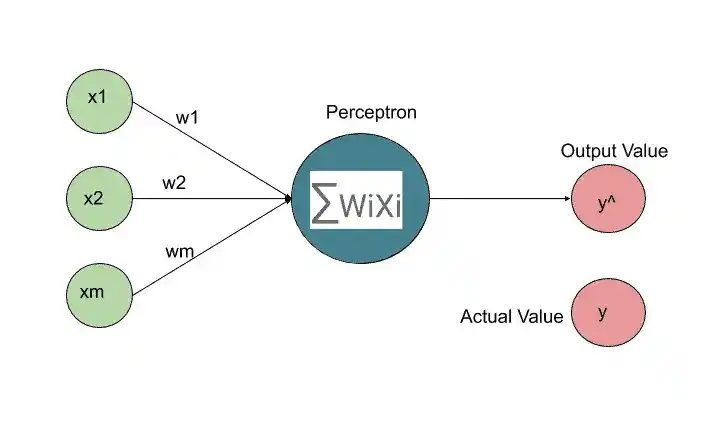
So, here we have some input values, that are supplied to the perceptron. Then the activation function is applied, and then we get an output. This output is y^. So the next step is that this predicted output is compared with the actual output y.
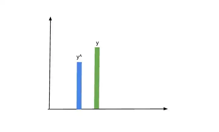
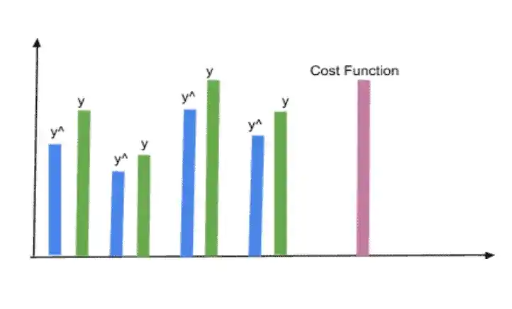
Suppose, we draw both outputs on this graph. And see how much they differ with each other.
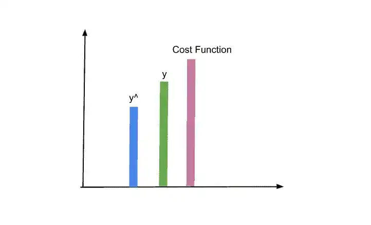
Now we calculate the cost function. This cost function is the square difference between the actual and predicted output. There are different cost function you can use. But the most commonly used cost function is –
cost function= 1/2 square(y – y^)
By calculating the cost function you can identify the error that you have in your prediction. And our goal is to minimize the cost function. The lower the cost function, the closer the predicted output is to the actual output.
After comparing the y and y^, we feed this information back into the neural network. So the weight gets updated.
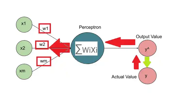
Basically, in a neural network, the only thing that we have control is weights. We update the weights and then on these weights the new output is predicted.
Again the cost function is calculated and we backpropagate to update the weights. This process continues until we get the predicted output the same or nearby as the actual output.
I want to clear one thing that all these processes are happening only for one row. Suppose you have to predict the student percentage based on how much he studies, sleep, and quiz percentage. So the study hour, sleep hour, and quiz percentage is the input value for the neural networks. But the whole process of learning happens for one student record something like that-
| RowID | Study Hrs | Sleep Hrs | Quiz | Exam |
|---|---|---|---|---|
| 1 | 10 | 7 | 80% | 90% |
So the learning process I have discussed with you is for that one record. Here Study Hrs, Sleep Hrs, and Quiz are the independent variables.
Based on these input variables we have to predict the Exam percentage. This 90% is the actual output that is y. So we feed these independent variables to the neural network, activation function is applied and then the output is generated.
We compare the predicted output with actual output with the help of the cost function. After that, we backpropagate and adjust the weights. This process continues until we get the predicted output of nearly y^ which is 90% in that case. Every time weights and y^ are changing.
So this the very simple case where I have shown you with the help of one row.
With Multiple Rows-
Now let’s see if there are multiple rows. Suppose you have a dataset with multiple rows something like that-
| Row Id | Study Hrs | Sleep Hrs | Quiz | Exam |
|---|---|---|---|---|
| 1 | 10 | 7 | 80% | 90% |
| 2 | 12 | 6 | 85% | 95% |
| 3 | 7 | 10 | 70% | 60% |
| 4 | 14 | 7 | 90% | 97% |
So to understand you properly, I just duplicate the same neural network four times.
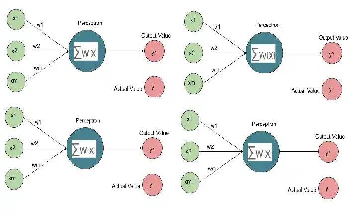
They are all the same perceptron, which is important to keep in mind. For each row, y^ is generated. And then we compare with the actual values. For every single row, we have an actual value. Based on the differences between all y^ and y, we can calculate the cost function. This cost function is for a full neural network.
Based on this cost function, we backpropagate and update the weights. One thing you should keep in mind is that this is one neural network, not 4. This is just to understand you properly.
So when we update the weights, we update the weights of one neural network. And the weights which we update are the same for all rows. Don’t think that weights are updated separately to each row.
The same process of learning can be performed with 4 rows as well as 400 rows.
What is the Gradient Descent Neural Network?
As we discussed how neural networks learn?. Its time to know What is Gradient Descent?
The cost function plays an important role in the neural network. So we need to optimize this cost function. The Gradient Descent works on the optimization of the cost function.
The one approach is the Brute Force approach, where we take all different possible weights and look at them to find the best one. But it is good if you have fewer weights, as the number of weights increases, or increases the number of synapses, you face the curse of dimensionality.
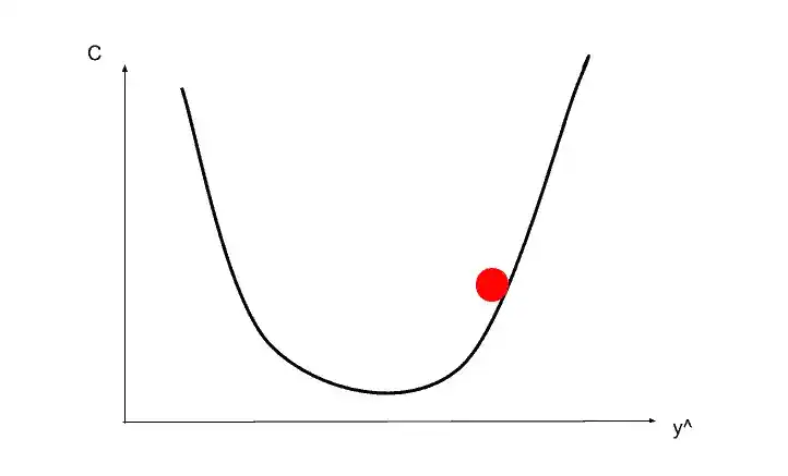
That’s why Gradient Descent is used to optimize the cost function. So to understand the gradient descent, let’s see in this image.
Suppose you start from this redpoint. So from that point in the top left, we are going to look at the angle of our cost function.
Here we are not going to discuss mathematical equations. Basically, you just need to differentiate and find out what the slope is in that specific point. And also find out if the slope is positive or negative. If the slope is negative like in the image, that means you are going downhill. so the right is downhill and the left is uphill.
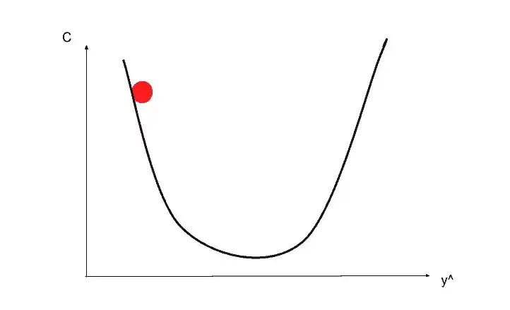
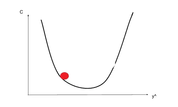
Suppose you go downhill and by rolling the redpoint come somewhere here.
Again calculate the slope, that time slope is positive meaning right is uphill and left is downhill so you need to go left. Something like that-
And again you calculate the slope and you need to move right. Here you go to the correct place. That’s how you find the best weights or the best situation that minimize the cost function.
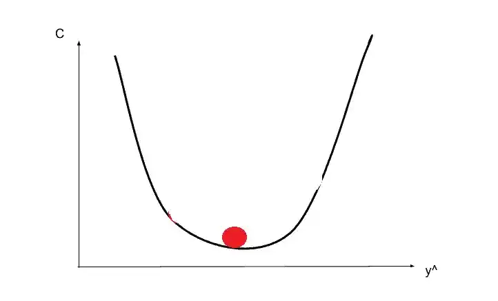
Of course, it’s not going like a ball rolling. It is going to be a very zigzag type of approach. But it is easy to remember and more fun to look at it as a ball rolling :-). In reality, it’s a step by step approach.
So that’s all about gradient descent. It’s called descent because you are descending or minimizing the cost function.
I hope now you understood What is Gradient Descent and How neural network learns. If you have any questions, feel free to ask me in the comment section. Read Stochastic Gradient Descent from here- Stochastic Gradient Descent- A Super Easy Complete Guide!
Enjoy Learning!
All the Best!
Thank YOU!
Though of the Day…
‘ It’s what you learn after you know it all that counts.’
– John Wooden
Read Deep Learning Basics here.

Written By Aqsa Zafar
Aqsa Zafar is a Ph.D. scholar in Machine Learning at Dayananda Sagar University, specializing in Natural Language Processing and Deep Learning. She has published research in AI applications for mental health and actively shares insights on data science, machine learning, and generative AI through MLTUT. With a strong background in computer science (B.Tech and M.Tech), Aqsa combines academic expertise with practical experience to help learners and professionals understand and apply AI in real-world scenarios.