Decision Tree in Machine Learning: A Complete Guide with Example

Do you wanna know about the Decision Tree in Machine Learning?. If yes, then this blog is just for you. Here I will discuss What is Decision Tree in Machine Learning?, Decision Tree Example with Solution?. So, give your few minutes to this article in order to get all the details regarding the Decision Tree.

Hello, & Welcome!

In this blog, I am gonna tell you-

Decision Tree in Machine Learning

In order to get all details regarding Decision Tree, first, start with the definition of a Decision Tree.

What is Decision Tree?

You might have heard the term “CART”. It stands for Classification and Regression Trees. That means it has two types of trees-

1. Decision Tree Classifier– Classification Tree help you to classify your data. It has categorical variables, such as male or female, cat or dog, or different types of colors and variables.
2. Decision Tree Regression– Regression Trees are designed to predict outcomes, which can be real numbers. For example the salary of a person, or the temperature that’s going to be outside.

That’s why Decision Tree is used in two places. Classification and Regression.

As the name suggests, “Decision Tree”, it is a Tree-shaped structure, which determines a course of action. Each branch in the Decision Tree represents a possible decision.

In Decision Tree, There are two nodes- Decision Node and Leaf Node.

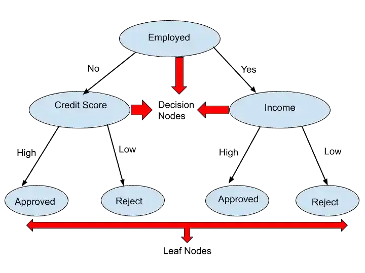
1. Decision Node– It is a node from where the branches of a tree grow. Based on the condition, these decision nodes decide the direction. In short, decision nodes are nothing but a Test. It tests the condition and then decides the direction. In that example of loan approval, at Employed Node, we test the condition. If the person is not Employed, then it comes under the second Decision node, which is a Credit Score. If the Credit Score is High, then Loan is approved.
2. Leaf Node- Leaf Nodes are the last nodes or the final nodes. In the Leaf node, we get our results. In that example, at a leaf node, we get to know that loan is approved or rejected based on the condition.

How does the Decision Tree work in Machine Learning?

To understand the working of the Decision tree, let’s take an example.

Suppose we have to classify different types of fruits based on their features with the help of the Decision Tree.

This is our dataset, which includes the color of fruit and the shape of the fruit. Based on these features, we can classify the type of fruits.

Color	Shape	Fruit Type
Red	Round	Apple
Orange	Round	Orange
Yellow	Long	Banana

Here, our Target variable is Fruit Type. Target Variable is nothing but a final result. So, here we have to classify the fruit type into different classes. That’s why our Target Variable is Type of Fruit.

Now we have to choose our Root Node. The Root node is the top node of a tree, from where the tree starts.

So, how we choose our Root Node?

To build a decision tree, we need to calculate two types of Entropy- One is for Target Variable, the second is for attributes along with the target variable.

1. The first step is, we calculate the Entropy of the Target Variable (Fruit Type).
2. After that, calculate the entropy of each attribute( Color and Shape).
3. After calculating the entropy of each attribute, find the Information Gain of each attribute (Color and Shape).
4. The attribute, who has high Information Gain, choose that attribute as a root node.

Now, you have a question What is Information Gain, Entropy, and Gain?

So, don’t worry. I will explain in the next section, where I will show you an example with a solution. Here I just gave you a brief idea of the Decision tree work procedure.

Now, Let’s see a solved numeric example of Decision Tree.

It’s not complicated. It’s fun.

Are you excited?

Yes.

Let’s start.

Decision Tree Example with Solution

Suppose we have the following dataset. In this dataset, there are four attributes. And on the basis of these attributes, we have to make a Decision Tree.

Age	Competition	Type	Profit
Old	Yes	software	Down
Old	No	software	Down
Old	No	hardware	Down
mid	yes	software	Down
mid	yes	hardware	Down
mid	No	hardware	Up
mid	No	software	Up
new	yes	software	Up
new	No	hardware	Up
new	No	software	Up

Step 1-

In that database, we have to choose one variable that is Target Variable. So in that dataset, choose Profit as a Target Variable.

Step 2-

Now, we have to find the Entropy of this Target Variable.

The formula of Entropy is-

Entropy= -[P/P+N log₂ (P/P+N) + N/P+N log₂ (N/P+N)]

Here, P is the number of “Down” in Profit, and N is the number of “Up” in Profit.

Up and Down are the values of Target Variable Profit.

So, Let’s calculate the Entropy for Target Variable (Profit)-

Down	Up
5	5

P= 5 (Number of “Down”), N = 5 (Number of “Up”), and P+N= 10.

Entropy= -[P/P+N log₂ (P/P+N) + N/P+N log₂ (N/P+N)]

= -[ 5/10 log₂ (5/10) + 5/10 log₂ (5/10) ]

= -[ 0.5x -1+ 0.5 x -1]

= -[ -0.5-0.5]

= -[-1]

= 1

Here, We get Information gain of our Target Variable as 1.

Step 3-

Now, we calculate the entropy of the rest of the attributes and that are- Age, Competition, and Type.

Let’s start with AGE.

Age attribute has 3 values- Old, Mid, and New.

Age	Down	Up
Old	3	0
Mid	2	2
New	0	3

Are you thinking, How I filled this Table?

So, Just have a look at the main dataset table.

where,

“Down” came 3 times in Old, that’s why I have written 3. And “Up” came 0 times in Old, that’s why it is 0.

Similarly “Down” came 2 times in Mid, and “Up” came 2 times in Mid.

And “Down” came 0 times in New, “Up” came 3 times in New.

Now, calculate the Entropy of Age attribute.

Entropy(Profit , Age)= Entropy(Old)+ Entropy(Mid)+Entropy(New)

Now, first, calculate the Entropy of Old-

P= 3 (“Down”), and N=0 (“Up”), P+N= 3,

Note- Probability (old)= Number of total old/ Total attributes = 3/10

Entropy(old) = -[P/P+N log₂ (P/P+N) + N/P+N log₂ (N/P+N)] x Probability(Old)

= -[3/3 log₂ (3/3) + 0/3 log₂ (0/3)] x 3/10

=0x 3/10

= 0

For Mid–

P= 2 (“Down”), and N=2 (“Up”) , P+N=4

Entropy(mid) = -[P/P+N log₂ (P/P+N) + N/P+N log₂ (N/P+N)]x Probability(Mid)

= -[2/4 log₂ (2/4) + 2/4 log₂ (2/4)] x 4/10

= 1×4/10

= 0.4

For New,

P= 0 (“Down”), and N=3 (“Up”) , P+N=3

Entropy(New) = -[P/P+N log₂ (P/P+N) + N/P+N log₂ (N/P+N)]x Probability(New)

= -[0/3 log₂ (0/3) + 3/3 log₂ (3/3)] x 3/10

= 0x3/10

= 0

Now, we have calculated the entropy of all 3 values of the Age attribute.

It’s time to add them.

Entropy(Profit , Age)= Entropy(Old)+ Entropy(Mid)+Entropy(New)

= 0 + 0.4 + 0

Entropy(Profit , Age) = 0.4

Now, we have calculated the entropy of Age Attribute.

Step 4-

Now we calculate the Information Gain of Age Attribute.

So, how to calculate the information gain?.

Let’s see.

The formula for calculating information gain is-

Information Gain(Target Variable, Attribute) = Entropy(Target Variable) – Entropy( Target Variable, Attribute)

So, calculate the information gain of Age Attribute-

Information Gain(Profit, Age) = Entropy(Profit)- Entropy(Profit, Age)

Information Gain(Profit, Age) = 1 – 0.4

Information Gain(Profit, Age) = 0.6

Now, we have finally calculated the information gain of Age Attribute. Similarly, calculate the information gain of the other two attributes- Competition, and Type.

I hope, you understood, how to calculate the information gain of attributes. That’s why I am directly taking the value of information gain of Competition and Type.

So, I have calculated the information gain of Competition and Type attributes. And the values are-

Information Gain(Profit, Age) = 0.6

Information Gain(Profit, Competition) = 0.124

Information Gain(Profit, Type) = 0

Step 5-

Now its time to choose the Root Node of the Decision Tree.

How to choose Root Node?

We choose the attribute as a root node, which has high information gain.

Now we know the Information Gain of all three attributes. Now we have to check, which attribute has high information gain.

So, after looking at all three values of information gain, we know that the Age attribute has high information gain.

That’s why we choose Age Attribute as Root Node.

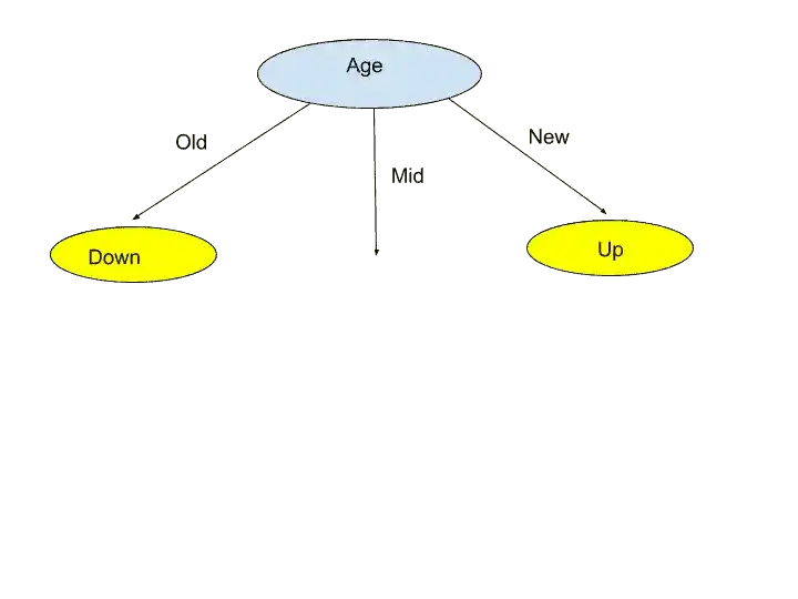
We have chosen the Age attribute as a Root Node. Now Age attributes have three values- Old, Mid, and New. That’s why we make three sections.

But, now you may be wondering, why I put Leaf Nodes as Down and Up in Old and New section.

So this is because, according to the main dataset, all the “Old” values are Down, No Old is in Up. That’s why it is easy to categories them in Down.

Similarly, all “New” values are in Up.

But, in “Mid”, there are 2 Down, and 2 Up. That means Mid is belonging to different sets of attributes. So whenever such a situation comes, we should take the next node.

So, how to choose the next node?

Again, the same method, the attribute who has high information gain, choose it.

So, in that case, the Competition attribute has high Information Gain as compare to Type attribute. That’s why Choose “Competition” as the next node.

The Competition attribute has two values- Yes and No. And according to the main dataset table, all the “yes” value belongs to “Down”, and the “No” value belongs to “Up”. That’s why “Yes” redirect to Down Leaf Node and “No” redirects to Up Leaf node.

And Here We Go!. We made our Decision Tree.

But,

You might be wondering that we didn’t use the “Type” attribute.

So the reason is, Type attribute has 0 information gain. And another reason is there is no need for the “Type” attribute. Without the “Type” attribute, we come to the Leaf node. And that is our goal.

If in “Competiton” attribute some “Yes” value point to “Down” and some point to “Up”, then we can take the Type Attribute for further classification. But here, this is not the case. That’s why we didn’t take Type attribute.

I hope now you understood the reason.

So, finally, we made our Decision Tree in the step by step manner.

Now, its time to see how we can implement a Decision Tree in Python.

Decision Tree in Python

To implement a Decision Tree Algorithm in Python, the first step is-

To import all required libraries-

import numpy as np
import pandas as pd
from sklearn.model_selection import train_test_split

The next step is-

To load the data–

dataset = pd.read_csv('Advertise.csv')
X = dataset.iloc[:, [2, 3]].values
y = dataset.iloc[:, 4].values

Here, we are calling the Panda library, therefore we write “pd.read_csv”. And inside pd.read_csv, we need to pass the file name in a single quote.

And We are storing the file values in the “dataset” variable.

We created two entities X and Y.

where X is metrics of features. And Y is the Dependent variable vector.

Metrics of feature or X is the values or attributes by which we predict or categorized.

Let me simplify it.

In the previous example, where we have three attributes, Age, Competition, and Type. So these are metrics of features or X. We use them to categorize the profit.

And Y or Dependent variables are nothing but the predicted or categorized value. In the previous example Profit is the Dependent variable or Y.

Got it?

That’s why, here in the code, we have divided our data into X and Y. And the value which we passed in the bracket are the column value of each attribute.

Depending upon your dataset, you can change these values. They are just for your reference.

Now, the next step is-

Split the Dataset into a Training set and Testing Set-

X_train, X_test, y_train, y_test = train_test_split(X, y, test_size = 0.2, random_state = 0)

We split our dataset into four variables- X_Train, X_Test, Y_Train, and Y_test.

train_test_split is a function that split our data into training and testing.

Here, we split 80% of data into Training Set, and 20% data into Test set.

So after slitting the Data, the next step is-

Perform Feature Scaling-

from sklearn.preprocessing import StandardScaler
sc = StandardScaler()
X_train = sc.fit_transform(X_train)
X_test = sc.transform(X_test)

We perform feature scaling because all the variables are not on the same scale. And it can cause some issues in your Machine Learning Model.

That’s why scaling is necessary to convert all values under the same range or scale.

We scale only the X variables.

The fit_transform method transform the normal variables into scaled variables.

Now, the next step is-

To Fit Decision Tree Classification to the Training set–

from sklearn.tree import DecisionTreeClassifier
dt = DecisionTreeClassifier(criterion = 'entropy')
dt.fit(X_train, y_train)

Here, we imported the DecisionTreeClassifier class. And inside DecisionTreeClassifier class, we only need to pass criterion as “entropy”.

After that, we train our Training data with Decision Tree algorithm by writing- dt.fit(X_train, y_train)

Once the model has been trained, the next step is-

Predict the Test set results

y_predict = dt.predict(X_test)

And this is the last step. After performing this step, you will get your results.

Here, I discussed the full implementation procedure in Python. I hope, you understood.

Conclusion-

In this article, you learned everything related to Decision Tree in Machine Learning.

Specifically, you learned-

1. How Decision Tree in Machine Learning works?
2. A step by step approach to solve the Decision Tree example.
3. How to implement the Decision Tree algorithm in Python.

I tried to make this article, “Decision Tree in Machine Learning” simple and easy for you. But still, if you have any doubt, feel free to ask me in the comment section. I will do my best to clear your doubt.

Enjoy Machine Learning

FAQ

All the Best!

Are you ML Beginner and confused, from where to start ML, then read my BLOG – How do I learn Machine Learning?

If you are looking for Machine Learning Algorithms, then read my Blog – Top 5 Machine Learning Algorithm.

If you are wondering about Machine Learning, read this Blog- What is Machine Learning?

Thank YOU!

Though of the Day…

‘ Anyone who stops learning is old, whether at twenty or eighty. Anyone who keeps learning stays young.

– Henry Ford