
In this article, I am gonna share the Implementation of Artificial Neural Network(ANN) in Python. So give your few minutes and learn about Artificial neural networks and how to implement ANN in Python.
So, without further ado, let’s get started-
- What is an Artificial Neural Network?
- ANN Implementation in Python
- 1. Data Preprocessing
- 1.1 Import the Libraries-
- 1.2 Load the Dataset
- 1.3 Split Dataset into X and Y
- 1.4 Encode Categorical Data-
- 1.5 Split the X and Y Dataset into the Training set and Test set
- 1.6 Perform Feature Scaling
- 2. Build Artificial Neural Network
- 2.1 Import the Keras libraries and packages
- 2.2 Initialize the Artificial Neural Network
- 2.3 Add the input layer and the first hidden layer
- 2.4 Add the second hidden layer
- 2.5 Add the output layer
- 3. Train the ANN
- 3.1 Compile the ANN
- 3.2 Fit the ANN to the Training set
- 4. Predict the Test Set Results-
- 5. Make the Confusion Matrix
- Conclusion
Implementation of Artificial Neural Network in Python
Before moving to the Implementation of Artificial Neural Network in Python, I would like to tell you about the Artificial Neural Network and how it works.
What is an Artificial Neural Network?
Artificial Neural Network is much similar to the human brain.
The human brain consists of neurons. These neurons are connected with each other. In the human brain, neuron looks something like this…
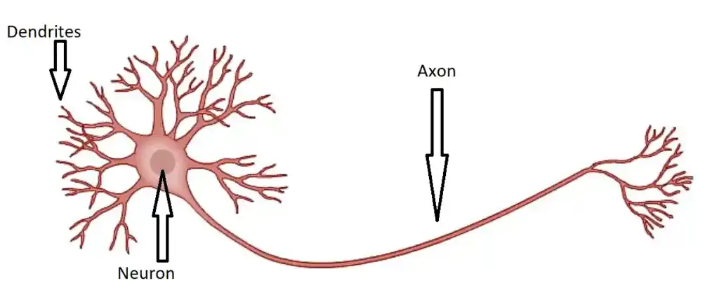
As you can see in this image, There are neurons, Dendrites, and axons.
Do you think?
When you touch a hot surface, how do you suddenly remove your hand? This is the procedure that happens inside you.
When you touch some hot surface. Then automatically your skin sends a signal to the neuron. And then the neuron takes a decision, “Remove your hand”.
So that’s all about the Human Brain. In the same way, Artificial Neural Network works.
Learn Artificial Intelligence with these-> 8 Completely FREE Courses to Learn AI (Artificial Intelligence)
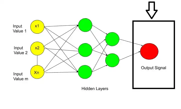
Artificial Neural Network has three layers-
- Input Layer.
- Hidden Layer.
- Output Layer.
Let’s see in this image-
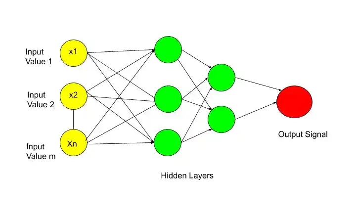
In this image, all the circles you are seeing are neurons. Artificial Neural Network is fully connected with these neurons.
Data is passed to the input layer. And then the input layer passed this data to the next layer, which is a hidden layer. The hidden layer performs certain operations. And pass the result to the output layer.
So, this is the basic rough working procedure of an Artificial Neural Network. In these three layers, various computations are performed.
Now Let’s understand each layer in detail. So the first layer is the Input Layer.
Input Layer
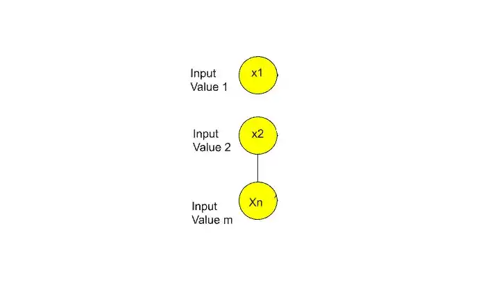
I think now you may have a question in your mind What signals are passed through the Input layer?
So in terms of the human brain, these input signals are your senses. These senses are whatever you can see, hear, smells, or touch. For example, if you touch a hot surface, then suddenly a signal is sent to your brain. And that signal is the Input signal in terms of the human brain.
But,
In terms of an artificial neural network, the input layer contains independent variables. So the independent variable 1, independent variable 2, and independent variable n.
The important thing you need to remember is that these independent variables are for one observation. In more simple words, suppose there are different independent variables like a person’s age, salary, and job role. So take all these independent variables for one person or one row.
Another important point you need to know is that you need to perform some standardization or normalization on these independent variables. It depends upon the scenario. The main purpose of doing standardization or normalization is to make all values in the same range. I’ll discuss this in the implementation part.
Now let’s move on to the next layer and that is-
Output Layer-
So, the next question is What can be the output value?
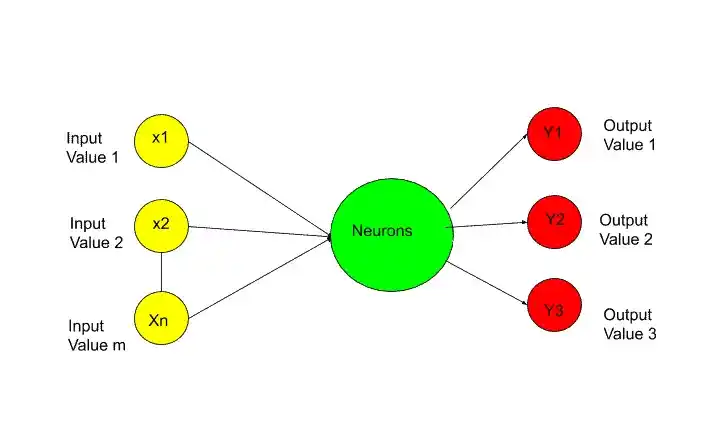
The answer is the output value can be-
- Continuous( Like price).
- Binary( in Yes/no form).
- Categorical variable.
Learn Artificial Intelligence with these-> 8 Completely FREE Courses to Learn AI (Artificial Intelligence)
If the output value is categorical then the important thing is, in that case, your output value is not one. It may be more than one output value. As I have shown in the picture.
Next, I will discuss synapses.
Synapses-
Synapses are nothing but the connecting lines between two layers.
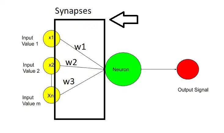
In synapses, weights are assigned to each synapse. These weights are crucial for artificial neural network work. Weights are how neural networks learn. By adjusting the weights neural network decides what signal is important and what signal is not important.
Hidden Layer or Neuron-
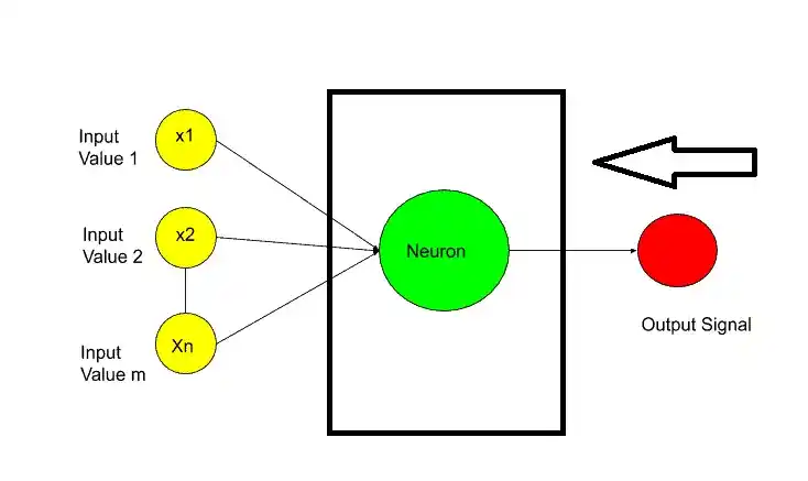
The next question is What Happens inside the neurons?
So Inside the neurons, the two main important steps happen-
- Weighted Sum.
- Activation Function.
The first step is the weighted sum, which means all of the weights assigned to the synapses are added with input values. Something like that-
[ x1.w1+x2.w2+x3.w3+………………..Xn.Wn]
After calculating the weighted sum, the activation function is applied to this weighted sum. And then the neuron decides whether to send this signal to the next layer or not.
I hope now you understood the basic work procedure of an Artificial Neural Network. Now let’s move to the implementation of Artificial Neural Network in Python.
Learn Artificial Intelligence with these-> 8 Completely FREE Courses to Learn AI (Artificial Intelligence)
ANN Implementation in Python
For implementation, I am gonna use Churn Modelling Dataset. You can download the dataset from Kaggle. Artificial Neural Networks can be used for both classification and regression. And here we are going to use ANN for classification.
This dataset has the following features-
This dataset has Customer Id, Surname, Credit Score, Geography, Gender, Age, Tenure, Balance, Num of Products they( use from the bank such as credit card or loan, etc), Has a Credit card or not (1 means yes 0 means no), Is Active Member ( That means the customer is using the bank or not), estimated salary.
So these all are independent variables of the Churn Modelling dataset. The last feature is the dependent variable and that is customer exited or not from the bank in the future( 1 means the customer will exit the bank and 0 means the customer will stay in the bank.)
The bank uses these independent variables and analyzes the behavior of customers for 6 months whether they leave the bank or stay and made this dataset.
Now the bank has to create a predictive model based on this dataset for new customers. This predictive model has to predict for any new customer that he/she will stay in the bank or leave the bank. So that bank can offer something special for the customers whom the predictive model predicts will leave the bank.
I hope now you understood the problem statement. So the first step in the Implementation of an Artificial Neural Network in Python is Data Preprocessing.
1. Data Preprocessing
In data preprocessing the first step is-
1.1 Import the Libraries-
import numpy as np
import matplotlib.pyplot as plt
import pandas as pd
NumPy is an open-source Python library used to perform various mathematical and scientific tasks. NumPy is used for working with arrays. It also has functions for working in the domain of linear algebra, Fourier transform, and matrices.
Matplotlib is a plotting library, that is used for creating a figure, plotting area in a figure, plotting some lines in a plotting area, decorating the plot with labels, etc.
Pandas is a tool used for data wrangling and analysis.
So in step 1, we imported all required libraries. Now the next step is-
1.2 Load the Dataset
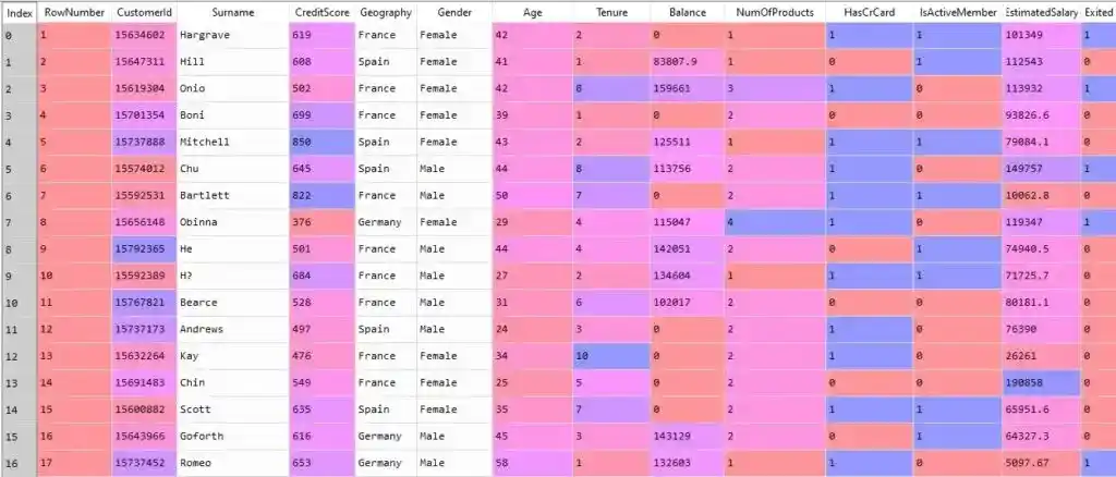
dataset = pd.read_csv('Churn_Modelling_dataset.csv')So, when you load the dataset after running this line of code, you will get your data something like this-
As you can see in the dataset, there are 13 independent variables and 1 dependent variable. But the first three independent variables Row Number, Customer Id, and Surname are useless for our prediction. So we will eliminate these three independent variables in the next step. And we will also split the independent variables in X and the dependent variable in Y.
1.3 Split Dataset into X and Y
X = pd.DataFrame(dataset.iloc[:, 3:13].values)
y = dataset.iloc[:, 13].values
Why dataset.iloc[:, 3:13].values? because credit_score has an index value of 3. And we want features from credit_score to estimated_salary.
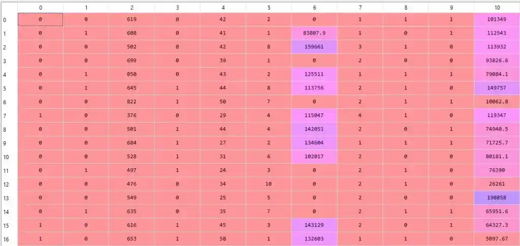
When you will run these lines, you will get two separate tables X and Y. Something like this-
Independent Variables (X)-
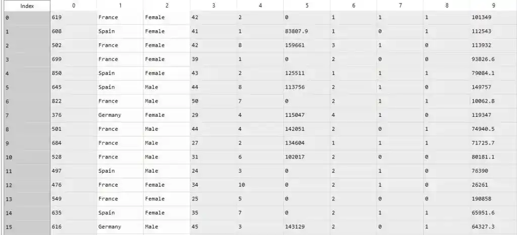
In this image, you can see that the dataset is starting from Credit_Score to the Estimated_Salary.
Dependent Variable(Y)–
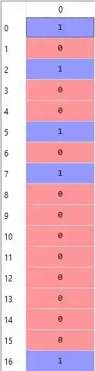
Now we have divided our dataset into X and Y. So the next step is-
1.4 Encode Categorical Data–
Why encoding is required…?
Because as we can see, there are two categorical variables-Geography and Gender. So we have to encode these categorical variables into some labels such as 0 and 1 for gender. And some hot encoding for geography variables.
So first let’s perform label encoding for gender variable-
from sklearn.preprocessing import LabelEncoder, OneHotEncoder
labelencoder_X_2 = LabelEncoder()
X.loc[:, 2] = labelencoder_X_2.fit_transform(X.iloc[:, 2])
Why I used 2…?
Because the Gender variable has an index value 2.
So after performing label encoding on the Gender variable, the male and female are converted into 0 and 1 something like this-
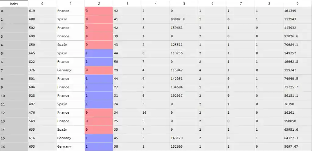
O represents the female and 1 represents the male. Now we have one more categorical variable and that is Geography. Now we will perform One hot encoding to convert France, Spain, and Germany into 0 and 1 forms.
One Hot Encoding-
First, we need to apply label encoding similarly to what we did in the gender variable. And then we will apply one-hot encoding. So, let’s have a look-
labelencoder_X_1 = LabelEncoder()
X.loc[:, 1] = labelencoder_X_1.fit_transform(X.iloc[:, 1])
After applying label encoding, now it’s time to apply One Hot Encoding-
onehotencoder = OneHotEncoder(categorical_features = [1])
labelencoder_X_1 = LabelEncoder()
X.loc[:, 1] = labelencoder_X_1.fit_transform(X.iloc[:, 1])
X = onehotencoder.fit_transform(X).toarray()
X = X[:, 1:]
So, when you run this code, you will get output something like this-
Confused after seeing the dataset…?
Let me explain,
Here [0 0] means- France.
[0 1] means Spain, and
[1 0] means Germany
So, the first two columns represent the Geography variable. I hope now you understood.
The next step is splitting the dataset into a Training and Test set.
1.5 Split the X and Y Dataset into the Training set and Test set
For building a machine learning model, we need to train our model on the training set. And for checking the performance of our model, we use a Test set. That’s why we have to split the X and Y datasets into the Training set and Test set.
from sklearn.model_selection import train_test_split
X_train, X_test, y_train, y_test = train_test_split(X, y, test_size = 0.2, random_state = 0)
While splitting into training and test set, you have to remember that, 80%-90% of your data should be in the training tests. And that’s why I write test_size = 0.2.
Now we have split our dataset into X_train, X_test, y-train, and y_test.
So the next step is feature scaling.
Learn Artificial Intelligence with these-> 8 Completely FREE Courses to Learn AI (Artificial Intelligence)
1.6 Perform Feature Scaling
As you can see in the dataset, all values are not in the same range, especially the Balance and Estimated_salary. And that requires a lot of time for calculation. So to overcome this problem, we perform feature scaling.
One thing you need to make sure of is always performing feature scaling in Deep Learning, no matter if you have already values in 0 forms.
Feature scaling helps us to normalize the data within a particular range.
from sklearn.preprocessing import StandardScaler
sc = StandardScaler()
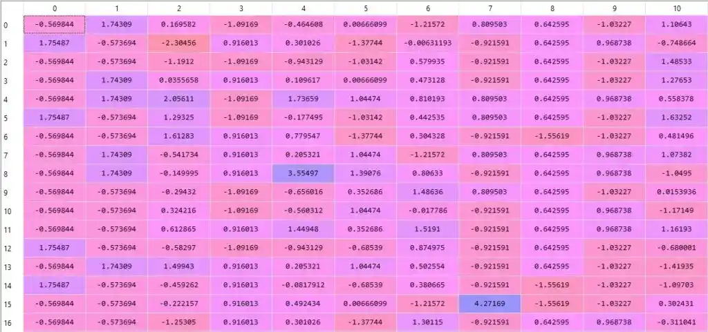
X_train = sc.fit_transform(X_train)
X_test = sc.transform(X_test)After performing feature scaling, all values are normalized and look something like this-
Now, we are done with the data preprocessing steps. Now it’s time to move to the second part and that is Building the Artificial Neural Network.
2. Build Artificial Neural Network
The first step is-
2.1 Import the Keras libraries and packages
import keras
from keras.models import Sequential
from keras.layers import Dense
2.2 Initialize the Artificial Neural Network
classifier = Sequential()The Sequential class allows us to build ANN but as a sequence of layers. As I told you in the theory part that ANN is built with fully connected layers. After initializing the ANN, it’s time to-
2.3 Add the input layer and the first hidden layer
classifier.add(Dense(output_dim = 6, init = 'uniform', activation = 'relu', input_dim = 11))Dense is a famous class in Tensorflow. Dense is used to add a fully connected layer in ANN.
“add” is the method in the Sequential Class. output_dim represents the number of hidden neurons in the hidden layer. But there is no rule of thumb for this. That’s why I used 6. You can use any other number and check.
The activation function in the hidden layer for a fully connected neural network should be the Rectifier Activation function. That’s why I use ‘relu’.
Our Input layer has 11 neurons. Why…?
Because we have 11 independent variables (including 2 columns of Geography).
That’s why input_dim = 11. Now we have built our first input layer and one hidden layer. In the next step, we will build the next hidden layer by just copying this code-
2.4 Add the second hidden layer
classifier.add(Dense(output_dim = 6, init = 'uniform', activation = 'relu'))Here again, we are using 6 hidden neurons in the second hidden layer. Now we have added one input layer and two hidden layers. It’s time to add our output layer.
2.5 Add the output layer
classifier.add(Dense(output_dim = 1, init = 'uniform', activation = 'sigmoid'))In the output layer, we need 1 neuron. Why…?
Because as you can see in the dataset, we have a dependent variable in Binary form. That means we have to predict in 0 or 1 form. That’s why only one neuron is required in the output layer.
And I write output_dim = 1.
The next thing is Activation Function. In the output layer, there should be a Sigmoid activation function. Why…?
Because the Sigmoid activation function allows not only predicts but also provides the probability of customers leave the bank or not.
For more details on Activation Functions, I would recommend you to read this explanation- Activation Function and Its Types-Which one is Better?
Now we have finally done with the creation of our first Artificial Neural Network. In the next step, we will train our artificial neural network.
3. Train the ANN
The training part requires two steps- Compile the ANN, and Fit the ANN to the Training set. So let’s start with the first step-
3.1 Compile the ANN
classifier.compile(optimizer = 'adam', loss = 'binary_crossentropy', metrics = ['accuracy'])compile is a method of Tensorflow. “adam’ is the optimizer that can perform the stochastic gradient descent. The optimizer updates the weights during training and reduces the loss. In order to understand the theory behind Gradient Descent, you can check this explanation-Stochastic Gradient Descent- A Super Easy Complete Guide!
One thing you need to make sure, of when you are doing binary prediction similar to this one, is always to use the loss function as binary_crossentropy.
For evaluating our ANN model, I am gonna use Accuracy metrics. And that’s why metrics = [‘accuracy’]. Now we have compiled our ANN model. The next step is-
3.2 Fit the ANN to the Training set
classifier.fit(X_train, y_train, batch_size = 10, nb_epoch = 100)Instead of comparing our predictions with real results one by one, it’s good to perform in a batch. That’s why I write batch_size = 10.
The neural network has to train on a certain number of epochs to improve the accuracy over time. So I decided the nb_epoch = 100. So when you run this code, you can see the accuracy in each epoch.
In the first epoch, the accuracy was-
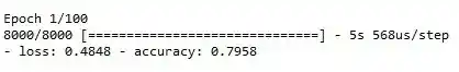
That is 79%, but after running all 100 epoch, the accuracy increase and we get the final accuracy-
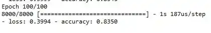
That is 83%. Quite good. Now we are done with the training part. The last but not least part is Predicting the test set results-
4. Predict the Test Set Results-
y_pred = classifier.predict(X_test)
y_pred = (y_pred > 0.5)
y_pred > 0.5 means if y-pred is in between 0 to 0.5, then this new y_pred will become 0(False). And if y_pred is larger than 0.5, then the new y_pred will become 1(True).
So after running this code, you will get y_pred something like this-
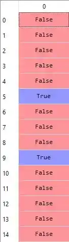
But can you explain by looking at these predicted values, how many values are predicted right, and how many values are predicted wrong?
For a small dataset, you can. But when we have a large dataset, it’s quite impossible. And that’s why we use a confusion matrix, to clear our confusion.
So, the next step is-
5. Make the Confusion Matrix
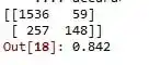
from sklearn.metrics import confusion_matrix, accuracy_score
cm = confusion_matrix(y_test, y_pred)
print(cm)
accuracy_score(y_test,y_pred)
And we got 84.2% accuracy.
That’s not bad. Now I would recommend you experiment with some values and let me know how much accuracy are you getting.
And here we go. Congratulation!
Learn Artificial Intelligence with these-> 8 Completely FREE Courses to Learn AI (Artificial Intelligence)
You have successfully built your first Artificial Neural Network. Now it’s time to wrap up.
Conclusion
I tried to explain the Artificial Neural Network and Implementation of Artificial Neural Network in Python From Scratch in a simple and easy-to-understand way. Hope you understood.
I would suggest you try it yourself. And if you have any doubts, feel free to ask me in the comment section. I would like to help you.
Happy Learning!
You May Also Be Interested In
10 Best Books on Neural Networks and Deep Learning, You Should Read
Deep Learning vs Neural Network, The Main Differences!
What is Generative Adversarial Network? All You Need to Know
Top 5 Deep Learning Algorithms List, You Need to Know
What is Convolutional Neural Network? Super Easy Explanation!
Top 6 Skills Required for Deep Learning That Will Make You Expert!
Stochastic Gradient Descent- A Super Easy Complete Guide!
Gradient Descent Neural Network- Quick and Super Easy Explanation!
How does Neural Network Work? A step by step Guide.
Activation Function and Its Types-Which one is Better?
Artificial Neural Network: What is Neuron? Ultimate Guide.
What is Deep Learning and Why it is Popular?
Thank YOU!
Though of the Day…
‘ It’s what you learn after you know it all that counts.’
– John Wooden
Read Deep Learning Basics Here

Written By Aqsa Zafar
Aqsa Zafar is a Ph.D. scholar in Machine Learning at Dayananda Sagar University, specializing in Natural Language Processing and Deep Learning. She has published research in AI applications for mental health and actively shares insights on data science, machine learning, and generative AI through MLTUT. With a strong background in computer science (B.Tech and M.Tech), Aqsa combines academic expertise with practical experience to help learners and professionals understand and apply AI in real-world scenarios.