SVM Implementation in Python From Scratch- Step by Step Guide

In this article, I am gonna share the SVM Implementation in Python From Scratch. So give your few minutes and learn about Support Vector Machine (SVM) and how to implement SVM in Python.

So, without further ado, let’s get started-

Read Also- Best Online Courses On Machine Learning You Must Know

SVM Implementation in Python From Scratch

Before moving to the implementation part, I would like to tell you about the Support Vector Machine and how it works.

What is a Support Vector Machine?

SVM was developed in the 1960s and refined in the 1990s. It becomes very popular in the machine learning field because SVM is very powerful compared to other algorithms.

SVM ( Support Vector Machine) is a supervised machine learning algorithm. That’s why training data is available to train the model. SVM uses a classification algorithm to classify a two-group problem. SVM focus on decision boundary and support vectors, which we will discuss in the next section.

How SVM Works?

Here, we have two points in two-dimensional space, we have two columns x1 and x2. And we have some observations such as red and green, which are already classified. This is linearly separable data.

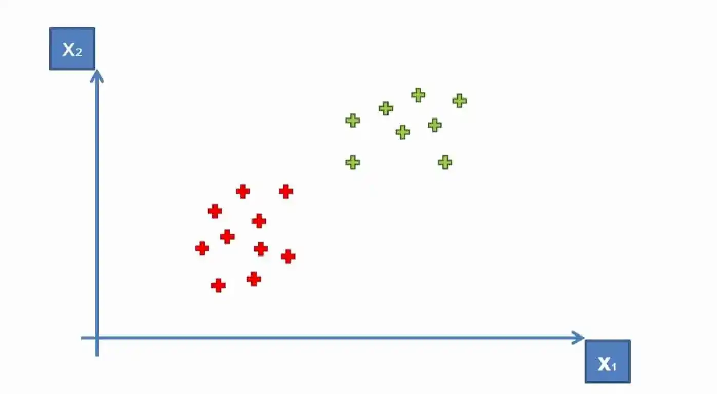
But, now how do we derive a line that separates these points? This means a separation or decision boundary is very important for us when we add new points.

So to classify new points, we need to create a boundary between two categories, and when in the future we will add new points and we want to classify them, then we know where they belong. Either in a Green Area or Red Area.

So how can we separate these points?

One way is to draw a vertical line between two areas, so anything on the right is Red and anything on the left is Green. Something like that-

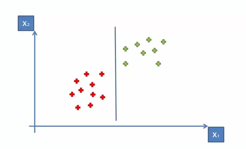
However, there is one more way, draw a horizontal line or diagonal line. You can create multiple diagonal lines, which achieve similar results to separate our points into two classes.

But our main task is to find the optimal line or best decision boundary. And for this SVM is used. SVM finds the best decision boundary, which helps us to separate points into different spaces.

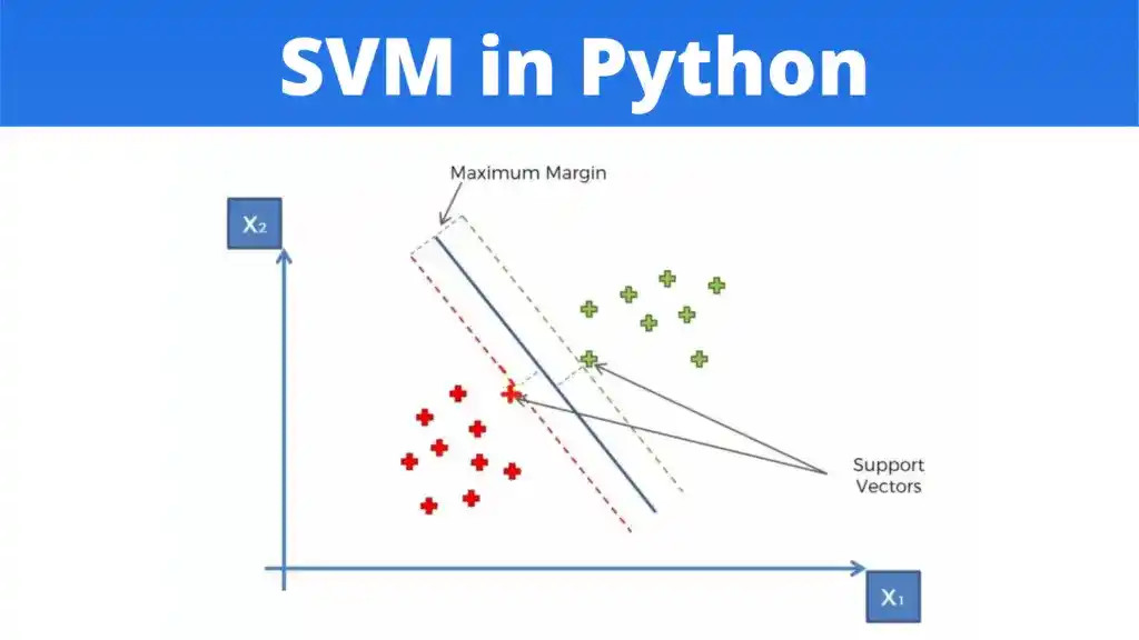
SVM finds the best or optimal line through the maximum margin, which means it has max distance and equidistance from both classes or spaces. The sum of these two classes has to be maximized to make this line the maximum margin.

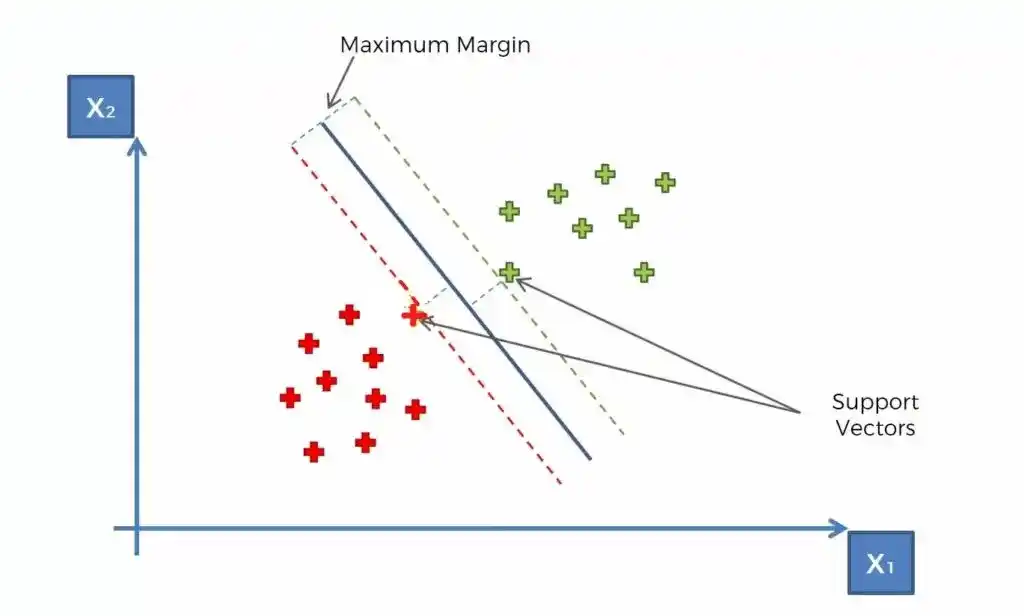
These, two vectors are support vectors. In SVM, only support vectors are contributing. That’s why these points or vectors are known as support vectors. Due to support vectors, this algorithm is called a Support Vector Algorithm(SVM).

In the picture, the line in the middle is a maximum margin hyperplane or classifier. In a two-dimensional plane, it looks like a line, but in a multi-dimensional, it is a hyperplane. That’s how SVM works.

Now let’s move to the SVM Implementation in Python From Scratch.

SVM in Python

Read Also- 10 Best Online Courses for Machine Learning with Python in 2024

For implementation, I am gonna use Social Network Ads Dataset. You can download the dataset from Kaggle. This dataset has two independent variables customer age and salary and one dependent variable whether the customer purchased SUVs or not. 1 means purchase the SUV and 0 means not purchase the SUV.

And we have to train the SVM model with this dataset and after training, our model has to classify whether a customer purchased the SUV or not based on the customer’s age and salary.

The first step is Data Pre-processing but before data pre-processing, we need to import the libraries. So let’s get started-

1. Import the Libraries-

import numpy as np
import matplotlib.pyplot as plt
import pandas as pd

NumPy is an open-source Python library used to perform various mathematical and scientific tasks. NumPy is used for working with arrays. It also has functions for working in the domain of linear algebra, Fourier transform, and matrices.

Matplotlib is a plotting library, that is used for creating a figure, plotting an area in a figure, plotting some lines in a plotting area, decorating the plot with labels, etc.

Pandas is a tool used for data wrangling and analysis.

So in step 1, we imported all required libraries. Now the next step is-

2. Load the Dataset

dataset = pd.read_csv('Social_Network_Ads.csv')

So, when you load the dataset after running this line of code, you will get your data something like this-

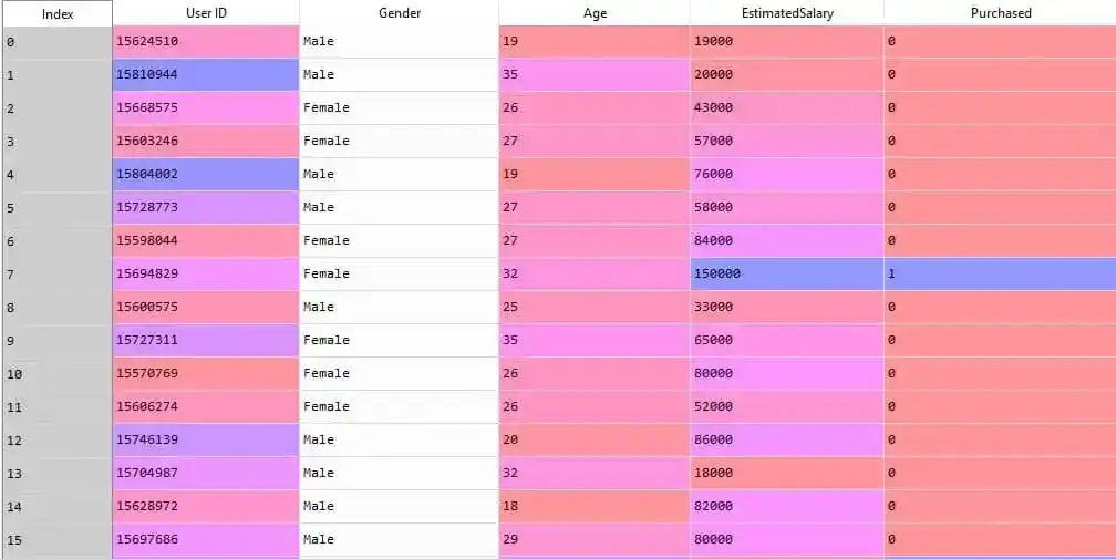
As you can see in the dataset, there 4 independent variables- UserID, Gender, Age, and Estimated Salary. And there is one dependent variable- Purchased.

But there is no need for UserID and Gender to this problem. In the next step, I will remove these two variables and split the dataset into X and Y. Here X represents independent variables and Y represents dependent variables.

3. Split Dataset into X and Y

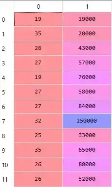
X = dataset.iloc[:, [2, 3]].values
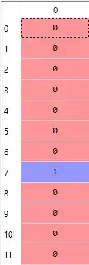
y = dataset.iloc[:, 4].values

When you run these lines, you get two separate tables X and Y. Something like this-

Independent Variables (X)-

Dependent Variable(Y)–

Now we have divided our dataset into X and Y. So the next step is-

4. Split the X and Y Dataset into the Training set and Test set

For building a machine learning model, we need to train our model on the training set. And for checking the performance of our model, we use a Test set. That’s why we have to split the X and Y datasets into the Training set and Test set.

from sklearn.model_selection import train_test_split
X_train, X_test, y_train, y_test = train_test_split(X, y, test_size = 0.25, random_state = 0)

While splitting into training and test set, you have to remember that, 80%-90% of your data should be in the training tests. And that’s why I write test_size = 0.25.

Now we have split our dataset into X_train, X_test, y-train, and y_test. The next step is-

5. Perform Feature Scaling

As you can see in the dataset, all values are not in the same range. And that requires a lot of time for calculation. So to overcome this problem, we perform feature scaling.

Feature scaling helps us to normalize the data within a particular range.

from sklearn.preprocessing import StandardScaler
sc = StandardScaler()
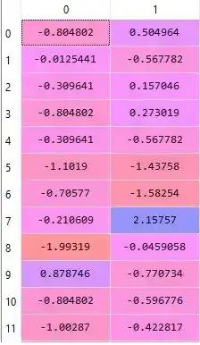
X_train = sc.fit_transform(X_train)
X_test = sc.transform(X_test)

After performing feature scaling, all values are normalized and looks something like this-

Now, we are done with the data preprocessing steps. It’s time to fit SVM into the training set.

5. Fit SVM to the Training set

from sklearn.svm import SVC
classifier = SVC(kernel = 'rbf', random_state = 0)
classifier.fit(X_train, y_train)

This SVC class allows us to build a kernel SVM model (linear as well as non-linear), The default value of the kernel is ‘rbf’. Why ‘rbf’, because it is nonlinear and gives better results as compared to linear.

The classifier.fit(X_train, y_train) fits the SVM algorithm to the training set- X_train and y_train.

Now, all done. It’s time to predict the Test set. So the next step is-

6. Predict the Test Set Results

y_pred = classifier.predict(X_test)

When you run this line of code, you will get y_pred, something like this-

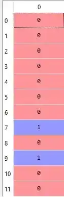
But can you explain by looking at these predicted values, how many values are predicted right, and how many values are predicted wrong?

For a small dataset, you can. But when we have a large dataset, it’s quite impossible. And that’s why we use a confusion matrix, to clear our confusion.

So, the next step is-

7. Make the Confusion Matrix

from sklearn.metrics import confusion_matrix, accuracy_score
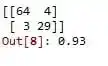
cm = confusion_matrix(y_test, y_pred)
print(cm)
accuracy_score(y_test,y_pred)

And we got 93% accuracy.

Now it’s time to showcase our findings in a visual form. So the next step is-

8. Visualise the Test set results

from matplotlib.colors import ListedColormap
X_set, y_set = X_test, y_test
X1, X2 = np.meshgrid(np.arange(start = X_set[:, 0].min() - 1, stop = X_set[:, 0].max() + 1, step = 0.01),
                     np.arange(start = X_set[:, 1].min() - 1, stop = X_set[:, 1].max() + 1, step = 0.01))
plt.contourf(X1, X2, classifier.predict(np.array([X1.ravel(), X2.ravel()]).T).reshape(X1.shape),
             alpha = 0.75, cmap = ListedColormap(('red', 'green')))
plt.xlim(X1.min(), X1.max())
plt.ylim(X2.min(), X2.max())
for i, j in enumerate(np.unique(y_set)):
    plt.scatter(X_set[y_set == j, 0], X_set[y_set == j, 1],
                c = ListedColormap(('red', 'green'))(i), label = j)
plt.title('SVM (Test set)')
plt.xlabel('Age')
plt.ylabel('Estimated Salary')
plt.legend()
plt.show()

So, after running this code, you will get your visual results-

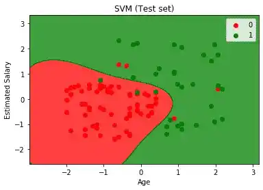
As you can see in the image, there are a total of 7 incorrect predictions. There are 3 green(Yes) predictions that were predicted as Red(No) and 4 Red(No) predictions that were predicted as Green(Yes).

But overall we got 93% accuracy and that’s great.

I hope now you have a better understanding of the Support Vector Machine. Now it’s time to wrap up.

Read Also- 15 Best+FREE Udacity Machine Learning Courses in 2024

Conclusion

I tried to explain SVM and SVM Implementation in Python From Scratch in a simple and easy-to-understand way. Hope you understood.

I would suggest you try it yourself. And if you have any doubts, feel free to ask me in the comment section. I would like to help you.

Happy Learning!

Thank YOU!

Though of the Day…

‘ Anyone who stops learning is old, whether at twenty or eighty. Anyone who keeps learning stays young.

– Henry Ford